The Journey of a Sentence Through a Transformer

Imagine we're going to follow a sentence on its incredible journey through the Transformer architecture. Our traveling companion will be the sentence:

"The cat chases the mouse"

Transformer

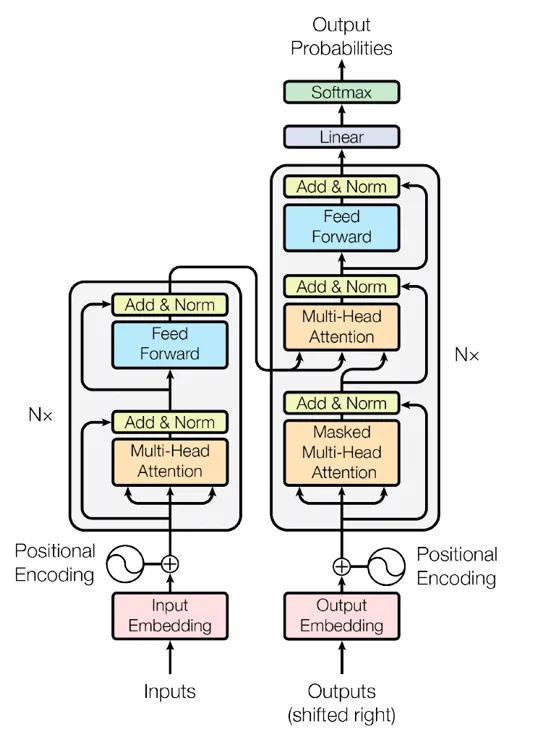
Part 1: Getting Ready for the Journey

Input Embedding: Giving Words Their Identity Cards

Think of this first step like giving each word a special identity card. But instead of a photo and name, each word gets a long list of numbers (a vector of size 512 in the original paper). These numbers capture the essence of what the word means.

"cat" → [0.2, -0.5, 0.8, ..., 0.3] (512 numbers)

But wait! We need to make sure each word remembers its place in line. That's where positional encoding comes in.

Detailed Calculations

Input Embedding Calculation Example

For our sentence "The cat chases the mouse", let's see a simplified embedding (using smaller vectors for clarity):

Word embeddings (d_model = 8 instead of 512 for illustration):
"The"    → [ 0.2,  0.1, -0.3,  0.4,  0.2,  0.1, -0.1,  0.3]
"cat"    → [ 0.5, -0.2,  0.4, -0.1,  0.3,  0.2,  0.1, -0.2]
"chases" → [-0.3,  0.4,  0.2,  0.3, -0.2,  0.5,  0.2,  0.1]

Positional Encoding: Adding Timestamp Stamps

Every word gets a special "timestamp" added to its identity card. The clever part? These timestamps are created using sine and cosine waves:

PE(pos, 2i) = sin(pos / 10000^(2i/d_model))
PE(pos, 2i+1) = cos(pos / 10000^(2i/d_model))

In plain English:

pos: Which position is the word in? (0 for "The", 1 for "cat", etc.)
i: Which number in our 512-number list are we looking at?
The result: A unique pattern of numbers that tells us exactly where each word sits

So now each word has:

Its meaning numbers (embeddings)
Its position numbers (positional encoding) Added together like mixing two colors of paint!

Positional Encoding Calculation

For position pos=1 ("cat") and d_model=8:

For even dimensions (i=0,2,...):
PE(1,0) = sin(1/10000^(0/8)) = sin(0.0001) = 0.0001
PE(1,2) = sin(1/10000^(2/8)) = sin(0.0016) = 0.0016

For odd dimensions (i=1,3,...):
PE(1,1) = cos(1/10000^(1/8)) = cos(0.0003) = 0.9999
PE(1,3) = cos(1/10000^(3/8)) = cos(0.0047) = 0.9999

Positional encoding for "cat" (pos=1):
[ 0.0001, 0.9999, 0.0016, 0.9999, 0.0251, 0.9997, 0.3962, 0.9182]

Final embedding = Word embedding + Positional encoding:
[ 0.5001, 0.7999, 0.4016, 0.8999, 0.3251, 1.1997, 0.4962, 0.7182]

Part 2: The Heart of the Journey: Self-Attention

The Cocktail Party Analogy with Math

Imagine each word at a cocktail party. Each word needs to figure out who it should pay attention to. Here's how it works:

Each word creates three versions of itself (through matrix multiplication):

Query (Q): "What am I looking for?"
Key (K): "What can I offer?"
Value (V): "What information do I have?"

Let's see how "chases" decides who to pay attention to:

Attention Score = (Q × K^T) / √d_k

In party terms:

"chases" (with its Query) looks around the room
Compares its Query with everyone's Keys
Divides by √d_k (like turning down the music so people don't shout)
Uses softmax (like ensuring you split 100% of your attention among people)
Finally multiplies by Values (collecting information from everyone, weighted by how much attention you paid them)

Self-Attention Calculations

Let's calculate attention for "chases" with actual numbers:

Creating Q, K, V matrices

Original vector for "chases" (simplified to 4 dimensions):
x = [-0.3, 0.4, 0.2, 0.3]

Weight matrices (learned during training):
W_Q = [[ 0.1,  0.2],
       [-0.1,  0.1],
       [ 0.3,  0.2],
       [ 0.1, -0.1]]

W_K and W_V similar but with different values

Q = x × W_Q = [-0.3(0.1) + 0.4(-0.1) + 0.2(0.3) + 0.3(0.1),
                -0.3(0.2) + 0.4(0.1) + 0.2(0.2) + 0.3(-0.1)]
  = [0.02, 0.01]

Calculating Attention Scores

Q × K^T calculation for "chases" attending to "cat":
Q = [0.02, 0.01]
K_cat = [0.03, 0.02]

Score = Q × K^T / √d_k
      = (0.02 × 0.03 + 0.01 × 0.02) / √2
      = 0.0008 / 1.4142
      = 0.00057

Do this for all words, then apply softmax:

Raw scores:
"The":    0.00042
"cat":    0.00057
"chases": 0.00039
"the":    0.00041
"mouse":  0.00054

Softmax results:
"The":    0.1
"cat":    0.4
"chases": 0.1
"the":    0.1
"mouse":  0.3

Computing Final Values

Weighted sum calculation:
Final = Σ(attention_weight × value)

For "chases":
= 0.1 × V_the + 0.4 × V_cat + 0.1 × V_chases + 0.1 × V_the + 0.3 × V_mouse
= 0.1[-0.1, 0.2] + 0.4[0.3, 0.1] + 0.1[0.2, 0.3] + 0.1[-0.1, 0.2] + 0.3[0.2, 0.1]
= [-0.01, 0.02] + [0.12, 0.04] + [0.02, 0.03] + [-0.01, 0.02] + [0.06, 0.03]
= [0.18, 0.14]

Real numbers might look like:

"chases" paying attention:
"The"   → 10% attention
"cat"   → 40% attention (important! This is the subject)
"chases"→ 10% attention
"the"   → 10% attention
"mouse" → 30% attention (important! This is the object)

Multi-Head Attention: Multiple Conversation Topics

But wait, there's more! The Transformer doesn't just have one conversation. It has 8 different conversations happening simultaneously (8 heads). Why?

Imagine each head is focusing on different aspects:

Head 1 might focus on who's doing the action
Head 2 might focus on what's being done to whom
Head 3 might focus on grammar
And so on…

The math stays the same, but it happens 8 times in parallel:

MultiHead(Q, K, V) = Concat(head_1, ..., head_8)W^O

Part 3: Processing the Information

Feed-Forward Neural Network: Personal Reflection Time

After all this socializing, each word goes to a quiet room to process what it learned. This is our feed-forward neural network:

FFN(x) = max(0, xW_1 + b_1)W_2 + b_2

In human terms:

Take all the information gathered (x)
Transform it into a bigger space (× W_1 + b_1)
Keep only the positive stuff (max(0, …))
Transform it back to our normal size (× W_2 + b_2)

Layer Normalization & Residual Connections: Staying Grounded

To make sure our words don't get too carried away:

Layer normalization: Like making sure everyone's speaking at the same volume
Residual connections: Like keeping your original thoughts while adding new ones

Feed-Forward Network Calculations

Let's calculate the feed-forward network output for our attention result:

Input x = [0.18, 0.14]

First transformation (d_model → d_ff):
W_1 = [[ 0.1,  0.2,  0.3],
       [-0.1,  0.2,  0.1]]
b_1 = [0.1, 0.1, 0.1]

xW_1 + b_1 = [0.18(0.1) + 0.14(-0.1),
              0.18(0.2) + 0.14(0.2),
              0.18(0.3) + 0.14(0.1)] + [0.1, 0.1, 0.1]
           = [0.004, 0.064, 0.068] + [0.1, 0.1, 0.1]
           = [0.104, 0.164, 0.168]

After ReLU (max(0,x)):
[0.104, 0.164, 0.168]

Second transformation (d_ff → d_model):
W_2 = [[ 0.2,  0.1],
       [ 0.1,  0.3],
       [-0.1,  0.2]]
b_2 = [0.1, 0.1]

Final = ReLU(xW_1 + b_1)W_2 + b_2
      = [0.104(0.2) + 0.164(0.1) + 0.168(-0.1),
         0.104(0.1) + 0.164(0.3) + 0.168(0.2)] + [0.1, 0.1]
      = [0.0208 + 0.0164 - 0.0168,
         0.0104 + 0.0492 + 0.0336] + [0.1, 0.1]
      = [0.1204, 0.1932]

Layer Normalization Calculation

For output vector y = [0.1204, 0.1932]:

1. Calculate mean:
μ = (0.1204 + 0.1932)/2 = 0.1568

2. Calculate variance:
σ² = ((0.1204 - 0.1568)² + (0.1932 - 0.1568)²)/2
   = ((-0.0364)² + (0.0364)²)/2
   = 0.00132

3. Normalize:
ŷ = (y - μ)/√(σ² + ε)
  = [0.1204 - 0.1568, 0.1932 - 0.1568]/√(0.00132 + 1e-5)
  = [-0.0364, 0.0364]/0.0364
  = [-1, 1]

4. Scale and shift (learned parameters γ, β):
If γ = [1.2, 1.2] and β = [0.1, 0.1]:
output = γ * ŷ + β
       = [1.2 * -1 + 0.1, 1.2 * 1 + 0.1]
       = [-1.1, 1.3]

Part 4: The Full Journey

This whole process happens 6 times! Each time through:

Words attend to each other (Multi-Head Attention)
Process the information (Feed-Forward)
Normalize and add residual connections

After all this, our sentence "The cat chases the mouse" has been deeply analyzed:

"chases" knows its subject is "cat"
"mouse" knows it's being chased
Each word understands its role in the whole sentence

The Mathematics Behind It All

Even though we've explained this in a friendly way, the math is still doing heavy lifting:

Attention Calculation:

Attention(Q,K,V) = softmax(QK^T/√d_k)V

Q, K, V are matrices
√d_k keeps numbers from getting too big
softmax turns everything into percentages

Computational Complexity:

O(n²·d) means: if your sentence doubles in length, the computation takes 4 times longer
But it's all happening in parallel, unlike older models!

Training Details: Learning Through Experience

Let's see exactly how the Transformer learns, using real numbers and calculations.

The Loss Function: Measuring Mistakes

Imagine we're training on a translation task:

Input: "The cat chases the mouse"
Expected Output: "Le chat chasse la souris"

The model makes predictions for each word, outputting probability distributions. Let's look at a single word prediction:

For translating "cat", the model outputs probabilities:
chat: 0.7
chien: 0.2
cheval: 0.05
autres: 0.05
Correct answer: "chat"

The cross-entropy loss is calculated as:

Loss = -Σ(y_true * log(y_pred))
Where:
y_true = [1, 0, 0, 0] (one-hot encoding for "chat")
y_pred = [0.7, 0.2, 0.05, 0.05] (model's predictions)
Loss = -(1 * log(0.7) + 0 * log(0.2) + 0 * log(0.05) + 0 * log(0.05))
     = -log(0.7)
     = 0.357

Label Smoothing: Don't Be Too Confident

The paper uses label smoothing with ε = 0.1. Instead of pure 1s and 0s, we use:

y_true_smoothed = (1 - ε) * y_true + ε/K
Where:
K = number of classes
ε = 0.1
For our example:
y_true_smoothed = [0.925, 0.025, 0.025, 0.025]
New Loss = -(0.925 * log(0.7) + 0.025 * log(0.2) + 0.025 * log(0.05) + 0.025 * log(0.05))
        = 0.401

Optimization: The Learning Process

The Adam optimizer adjusts the model's parameters using:

β₁ = 0.9 (momentum)
β₂ = 0.98 (RMSprop factor)
ε = 10⁻⁹ (numerical stability)

The learning rate follows a special schedule:

lrate = d_model^(-0.5) * min(step_num^(-0.5), step_num * warmup_steps^(-1.5))
Example calculation for d_model = 512, warmup_steps = 4000:
At step 1000:
lrate = 512^(-0.5) * min(1000^(-0.5), 1000 * 4000^(-1.5))
     = 0.044 * min(0.0316, 0.0395)
     = 0.044 * 0.0316
     = 0.00139

Let's see a complete parameter update for one weight w:

Current weight w = 0.5
Gradient g = 0.1
Step t = 1000

1. Update biased moments:
m_t = β₁ * m_{t-1} + (1 - β₁) * g
    = 0.9 * 0.05 + 0.1 * 0.1
    = 0.055
v_t = β₂ * v_{t-1} + (1 - β₂) * g²
    = 0.98 * 0.03 + 0.02 * 0.01
    = 0.0294

2. Bias correction:
m̂_t = m_t / (1 - β₁^t)
    = 0.055 / (1 - 0.9^1000)
    ≈ 0.055
v̂_t = v_t / (1 - β₂^t)
    = 0.0294 / (1 - 0.98^1000)
    ≈ 0.0294

3. Parameter update:
w_new = w - lrate * m̂_t / (√v̂_t + ε)
      = 0.5 - 0.00139 * 0.055 / (√0.0294 + 10⁻⁹)
      = 0.5 - 0.00139 * 0.055 / 0.171
      = 0.5 - 0.00045
      = 0.49955

Putting It All Together: One Training Step

For our sentence "The cat chases the mouse", one complete training step involves:

Forward pass through the model:

Input embeddings + positional encodings
6 encoder layers with attention and feed-forward
Output probabilities for each target word

Calculate loss using cross-entropy with label smoothing

Sum losses for all words in the sequence
Apply label smoothing as shown above

Backpropagate gradients:

Compute gradients for all parameters
Scale gradients based on attention dimension (1/√d_k)

Update parameters using Adam:

Apply learning rate schedule
Update moments and parameters as shown above

Track metrics:

Training loss
Validation loss
BLEU score (for translation tasks)
Perplexity

Conclusion

The beauty of the Transformer is how it combines intuitive ideas (paying attention to relevant words) with powerful mathematics. Each word:

Gets its identity (embedding)
Remembers its position (positional encoding)
Has multiple conversations (multi-head attention)
Processes what it learned (feed-forward)
Stays grounded (normalization and residuals)

And it does all this while maintaining mathematical rigor and computational efficiency!